The Last Guide to VLOOKUP You’ll Ever Need
This Guide was provided by http://spreadsheeto.com/vlookup/ from Hannah Sharron, Great job!
VLOOKUP is one of the most well-known Excel functions – and not without reason!

VLOOKUP’s ease of use and simplicity when “looking up†data is unparalleled in Excel.
- Maybe you want to learn the basics of VLOOKUP step-by-step?
- Perhaps your VLOOKUP formula isn’t working?
If yes, then you’ve come to the right place!
This is the definitive guide to VLOOKUP.
Using VLOOKUP
“A VLOOKUP simply looks for something in a range of cells and returns something that’s in the same row as the value you are looking for.â€
The only caveat is, that the datasheet has to be listed vertically (which is the case 99% of the time).
To help you better understand the power of VLOOKUP, we’ve created a sample file with a list of employees. With this data in hand, we’re going to create a tool that searches this list of employees and return the specific data we’re looking for – all powered by VLOOKUP.
Therefore, go ahead and download our free sample file below, open it and follow along…
*I highly encourage you to download our free sample file just above, as this tutorial will be based on the data provided in the sample file.
Got the sample file? And opened? Awesome, then you’re good to go!
Let’s say you’re looking for Nate Harris’ salary.
It would be a waste of time to look for his name in column A manually and then (again) manually typing his salary in the cell you need it to be in.
VLOOKUPÂ can do the trick in less than 1 minute.
Let’s build a tool where you can enter an employee’s name and then automatically see his or her salary in a matter of seconds.
Building a machine like this is split up in 6 (easy) steps.
Therefore, every time you need a VLOOKUP function, use these 6 steps below.
Luckily, this process isn’t nearly as sophisticated as it may sound.
Now, let’s take a closer look at our sample file.

Step 1: A place for your formula
Most people just put formulas into random cells. Don’t be that person!
I find that this usually ends in “spreadsheet mayhem†(not good!) and is ultimately the cause of death for the workbook.
Why?
Because the calculations and data storage get mixed up. It can be revived, but usually, it’s easiest to start over.
If you don’t want to start over after several months of hard work in a workbook – do get the structure of your calculations and data right from the beginning.
There are several ways of doing this, with some being more complicated (and effective) than others.
In the following, you’ll find my approach to creating a VLOOKUP which has been fine-tuned over several years and for me is the easiest and fastest solution.
Let’s take the first steps…
Select some cells where you want the result of your calculation (the VLOOKUP function) to go.
We’re going to be looking for something, so include a spare cell to use for “searchingâ€.
In this case 4 cells in total. Two for the name and two for the salary.
- Select cells E2:F3. Go to the “Font†group of the “Home†tab on the ribbon and click the little arrow next to the “Borders†button.
- Right click and select “Format Cellsâ€. Then go to the “Border†tab.
- Select a thick border from the “Style†options and click on the “Outline†preset. Then click the horizontal line in the mid of the example.
- Now select a thinner border style and click the vertical line in the mid of the example.
- Type in “Name†in cell E2 and “Salary†in E3 and make the text bold.
Or watch the animation below.

Now we have a pretty little area to fill in what we’re looking for (cell F2) and our formula with VLOOKUP below (cell F3).
That was pretty simple, right?
It’s already time to move on to your next step!
Step 2: What are you looking for?
Now it’s time to get into the syntax of VLOOKUP.
“Syntax†is just a big ugly word that doesn’t make much sense unless you’ve heard it before.
But what it means is actually really simple.
“Syntax is a combination of the things you need to put into a function to make it work.â€
A VLOOKUP function needs these 4 inputs in order to work:
- Lookup_value = What you are looking for
- Table_array = Where you are looking
- Col_index_num = What we want to know
- [range_lookup] = Whether we want to be precise or approximate in our search
When we start entering the formula in a moment, you’ll see all of these phrases inside a tooltip box below the cell you’re typing in.
All these inputs to the VLOOKUP formula must be separated with a comma (like in most other functions).
Every time you put a comma, the tooltip box tells you how far you are in the formula, by bolding the current part of the syntax.
But enough with all the technicalities!
Imagine the VLOOKUP function doing the same as you when you want to look something up.Â
 I know phonebooks are pretty outdated by now, but let’s say that we’re using one right now.
- You’re looking for Nate Harris’ salary. A proper phonebook may not contain that kind of information but for the sake of this example – let’s say it does.
- You acknowledge that we’re looking for the name ‘Nate Harris’ in the phonebook. This is your identifier. The piece of information you’re searching for with your eyes. In Excel terms, this is your lookup value.
- You browse through the pages and find Nate Harris. You place the tip of your finger right below his name and move your hand to the right past information like his address, phone number and other boring stuff. And there you have it! His salary! 3 inches to the right of his name. Then you write it down or do whatever you want to do with it.
That’s exactly how a VLOOKUP works!
So our lookup value is typed into cell F2 and then used in our function.
I guess you’re getting the point by now? So let’s start building the formula!
Type this into Excel in cell F3 (also shown in the screenshot right below):
=VLOOKUP(

And what comes next is the name of the employee we want to find more information about.
As a lookup value, you can either type in the name (“Nate Harrisâ€) or put in a reference to the cell where you’ll type in the name.
The last option is usually the best and our sheet is setup to have the name entered in cell F2.
So we’re going to select cell F2 (or type F2 in the formula bar) and type a comma to move on in the formula.

In this case, the VLOOKUP formula will not be copied, but the sheet structure might be changed at some point.
To prevent the formula from being messed up, we lock the reference to cell F2.
This is achieved by putting the marker inside (or around) the F2 and pressing the shortcut F4 (on MAC: Command + T). Like done below:

Your formula now looks like this:

Step 3: Where are you looking?
This step is where we are looking for our guy Nate.
When you are looking for Nate Harris manually (using your eyes, not your awesome Excel skills), where do you look?
Well, Excel “looks†almost the same place.
So we’re looking in column A of the data – the one called ‘Full Name’ – Excel is also looking in column A with its creepy computer eyes.
However, the VLOOKUP function needs to know the entire dataset in order to return the information you want later on in step 4.
So select (or type) range A2 through C55 and press F4 (MAC: Cmd + T).
Now the reference to the range is locked and you can move on to the next step by typing a comma.
Your formula should look like this:

Step 4: What you want to return
When you use a VLOOKUP formula you want an answer to something.
What you want to return is what Excel calls the col_index_num (Column Index Number).
In short: Which column in the data you want to return data from.Â
When you’re looking for Nate Harris and find him in row 17 of the sample data, the column index number determines which column in the data the result will come from.
It’s as simple as this.

Column A has Column Index Number 1, column B has 2 and column C has 3.
That seems pretty straightforward, but you need to be aware of following:
The column index number is relative to the data you selected in step 3.Â
You selected the cells A2 through C55. That means that the data stretches 3 columns wide.
In this case, we want to return data from Column C which is column index number 3. But if the data was located differently in our Excel sheet, then column C would not have column index number 3.
Look at the picture below.
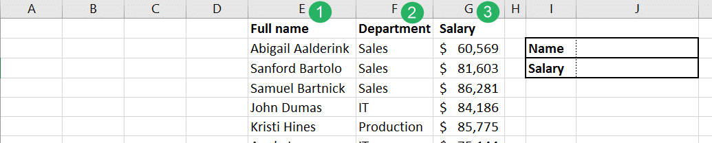
In this example where I’ve moved the data 4 columns to the right, column E is now column index number 1, column F is 2 and column G is 3.
Column A, B, C, D and all the other columns to the right of the data are now not considered a part of the data and have no column index numbers.
Got it? Great!
Going back to our original data in the sample file, you want to return the salary which is located in column index number 3.
Simply type 3 in your formula and move on to the next step by typing a comma.
Your formula should now look like this.

Let’s move on to the next step.
Step 5: Do you want to be precise or approximate?
When we look for something like a name (Nate Harris) and want to see his salary we don’t want to find a Nathan Jones or a Nate Miller instead just because their names are close to each others.
Excel deals with these 2 terms:
| “Approximate match†| “Exact match†|
|---|---|
| Used if you’re looking for a value that is closest to your lookup value. | Used if you’re looking for a value that is equal to your lookup value. |
It’s very easy to choose whether to use EXACT or APPROXIMATE match.
Just pick “FALSE†from the helper menu that pops up when you’ve entered the comma from the step 4 – alternatively, you can type ‘FALSE’ after the comma.
Your formula should look like this by now.

Rule of thumb: Always pick “exact match†when using VLOOKUP
But rules are made to be broken right?
The exception: When you’re looking for a value inside an interval you can use VLOOKUP with approximate match.
This is better illustrated by using an example, so let’s imagine a dataset like this:
The Exception: When to use “approximate matchâ€

When the lookup value is 15 (which it is in the picture) the ware status in cell E4 (where the formula is) shows ‘Very low’.
In this example, the values are categorized like this:
- 1-19 equals a very low status.
- 20-39 equals a low status.
- 40-59 equals medium.
- 60-79 equals high.
- 80+ equals very high.
In this case, you can’t use a VLOOKUP formula with EXACT match since this would only work when the quantities 0, 1, 20, 40, 60 and 80 are entered in the lookup value cell (E4).
With the data set up in intervals like this, you want to use VLOOKUP with approximate match (in almost every other scenario you should go for the exact match).
Great, so that is when you should use “approximate match†instead of “exact matchâ€.
Now, let’s continue with the primary example of this article.
Let’s put a parenthesis and get on with our formula.
It should look like this:

It’s time to move on to the last step…
Step 6: Press enter
What do we usually do when completing a formula?
We press enter.
And that’s exactly what you’re going to do now!

When you’ve pressed “Enter†we actually don’t know if the formula is working or not.
We have to enter something the formula can look for in the ‘lookup value cell’ (F2) to validate what we’ve done is correct (which is why you’re currently seeing a #N/A error).
At the #N/A error, click the small exclamation mark left to the cell and you can see that Excel calls this a ‘Value Not Available Error’.
When we haven’t entered anything as the lookup value, Excel is automatically looking for ‘nothing’ in the left column of the table array.
When it can’t find anything (there’re only cells that contain something in our table array), it simply returns an error that states that it can’t find what you’re looking for.
Let’s try and type Nate Harris into our ‘Name’ cell (F2) and see what happens…

Congratulations!
You’ve now made a tool to search for a person’s salary in an employee table.Â
Try to enter other people’s names in the ‘lookup value’ cell (F2) and witness the power of your newly created tool.
Sadly, creating a VLOOKUP formula can go wrong sometimes.
How do you fix it?
Read on and learn how to troubleshoot your VLOOKUP formula.
VLOOKUP not working? Here’s how to fix it!
There can be multiple reasons why your VLOOKUP formula isn’t working the way you want it to.
Most of the mistakes derives from forgetting how VLOOKUP works and/or mismatches in the data.
All of these result in an error (mostly #N/A or #REF!).
In the following I will walk you through the most common reasons why your VLOOKUP formula is not working as intended.
The infamous #N/A error
When your VLOOKUP formula returns #N/A it means that the value you’re searching for is not available.
Fear not! One of the following steps will fix your formula.
1. Typos or additional spaces in your lookup value
If you’ve spelled the name you’re looking up incorrectly, or accidentally entered an additional space somewhere in the lookup value, VLOOKUP won’t work.
To ensure that you haven’t, do the following:
- Double click the lookup value
- Place your marker in the beginning of the value and press backspace
- Do the same at the end of the value
Above process is also shown in the animation below.

2. Typos or additional spaces in the lookup data
If your lookup value is correct, but the formula still results in a #N/A error, it might be because the data you’re looking in is filled with typos or extra spaces.
In my experience, this is a common issue when data is copy/pasted from another sheet, file type or program.
The typos you probably have to take care of manually unless you can identify some kind of system in the typos.
If you’re lucky you can ‘search and replace’ the typos.Â
This applies to you if you always misspell something like the name Kristi, and need to change all instances of Kristi with Christy.
Here’s how to fix it:
Press the shortcut Ctrl + H (MAC: ^ + H) to bring up the ‘search and replace’ box and enter the way you’ve spelled it in the ‘Find what:’ field.
Then enter what you want to replace it within the ‘Replace with:’ field.
If you wanted to replace Kristi with Christy, you’d just have to set it up like this:

Regarding the additional spaces in front of or after (or both) the values, this can easily be solved by using the “TRIM functionâ€.Â
Follow these 6 easy steps, to get rid of any unnecessary spaces.
- Make a helper column anywhere you want – for example in column H.
- In cell H2 type in the formula: =TRIM(A2)
- Drag it down to the rest of the rows so it matches the content of column A.
- Now select all the formulas in column H and copy them.
- Select cell A2, right click and hover your mouse over ‘Paste’. Then click ‘Values’.
- Delete all the content of column H.
Now the cells in column A (your lookup column) has no excess spaces and is ready to be ‘looked’ in by the VLOOKUP formula.
If this does not fix your error-issues, read on.
3. The column with lookup values is not farthest to the left in your lookup table.
This is an important issue to notice as it’s the very foundation of a successful VLOOKUP.
The column in which you’re looking for your lookup value must be the leftmost column in your lookup table.Â
VLOOKUP looks in the left side of the table and returns things to the right of the lookup value when it finds it.


So if you’ve structured your data in another way, you should consider restructuring it so the lookup column is to the left of the column where you want to return values from.
4. Numbers formatted as text
If you’re looking for numbers in a list with numbers, you should make sure they are not formatted as text.
This can happen from time to time, but is easily fixed.
Excel will identify numbers formatted as text and come up with a warning. If you click on it, you can make Excel convert the text to a number with a single click.

The #REF error
This type of error comes from one of two issues.
1. Column Index Number is greater than number of columns
The table array (the data you’re looking in) is not as big as what you’re telling Excel in the VLOOKUP syntax (Column Index Number).
If your table array is 3 columns wide, like it is in this case, and you want a successful lookup to return values from the 4th column you’re doing something wrong. Excel tells you this by showing a #REF error as a result.

If we change the ‘Column Index Number’ to 3 instead of 4 it matches with the number of columns in our table.

2. The references in the VLOOKUP formula points to cells that no longer exists.
We use the lookup value to tell Excel what we’re looking for.
When we use our VLOOKUP tool we often design it so the result is very close (physically) to the lookup value in our spreadsheet.
We do this to save some time and don’t waste any looking for the result of our lookup. That means that we tend to forget where VLOOKUP actually looks to “fetch†us some numbers.
If the table array (the place where VLOOKUP fetches the result) is somehow deleted or moved, then our VLOOKUP formula will return a #REF! error because a reference in the formula doesn’t work any longer.
Even if you put new numbers in the table array, the formula will still no longer work – since the references have been destroyed.
In order to trigger this error, it is not enough to just select the table array and press the ‘Delete’-key.
You have to select the table array and press ‘Delete’-button on the ‘Home’-tab. Then press ‘Delete cells’.

When the cells are removed like this, the references will be destroyed and you’ll get an #REF! error.

If you just delete the content of the cells in the table array, you’ll get a #N/A error – because the values cannot be found anymore.

This is how you troubleshoot the most common issues when using VLOOKUP.
So you’ve now learned how to create a VLOOKUP in 6 easy steps and how to troubleshoot your VLOOKUP if it’s not working.
